import pandas as pd #분석 사용
import numpy as np #수치 계산
import seaborn as sns #시각화 사용
import matplotlib.pyplot as plt # 그래프 시각화

#%matplotlib inline # 구버전의 주피터 노트북에서 설정이 되어야 노트북 안에서 그래프가 시각화 된다5: 건강검진 데이터로 가설검정
부스트코스
음주 여부에 따라 건강검진 수치 차이가 있을까?
신장과 허리둘레의 크기는 체중과 상관관계가 있을까?
라이브러리 로드
한글폰트 설정
# Google colaboratory을 사용할 경우는 ctrl(cmd) + /로 주석을 없애서 실행을 합니다.


# Jupyter notebook을 사용할 떄는 다음과 같이 코드를 작성합니다.

# 마이너스 폰트가 깨지는 문제를 대처하기 위해 아래 코드를 작성합니다.
import os
# 윈도우, 맥 외의 os는 별도로 설정

if os.name == 'posix' :
    plt.rc("font", family="AppleGothic")
else:
    plt.rc("font", family="Malgun Gothic")

    # 마이너스 폰트 깨지는 문제 대처
plt.rc("axes", unicode_minus=False)
# 레티나 설정시 글씨가 좀 더 선명하게 보인다.
# 폰트의 주변이 흐릿하게 보이는 것을 방지한다.
%config InlineBackend.figure_format = 'retina'데이터 불러오기
- 국민건강보험 데이터를 사용하겠습니다. 공공데이터포털에서 건강검진정보를 다운로드 받습니다. 우리가 엑셀도 좋지만 파이썬으로 데이터 분석을 배우는 이유는 대용량 데이터를 분석하기 위함입니다. 2018년 데이터는 utf-8로 되어 있고, 2017년 데이터는 한글 인코딩이 되어 있습니다. 2017년 데이터를 사용합니다.
df=pd.read_csv("data/NHIS_OPEN_GJ_2017.CSV", encoding="cp949")
df| 기준년도 | 가입자일련번호 | 성별코드 | 연령대코드(5세단위) | 시도코드 | 신장(5Cm단위) | 체중(5Kg 단위) | 허리둘레 | 시력(좌) | 시력(우) | ... | 감마지티피 | 흡연상태 | 음주여부 | 구강검진 수검여부 | 치아우식증유무 | 결손치유무 | 치아마모증유무 | 제3대구치(사랑니)이상 | 치석 | 데이터공개일자 | |
|---|---|---|---|---|---|---|---|---|---|---|---|---|---|---|---|---|---|---|---|---|---|
| 0 | 2017 | 1 | 1 | 13 | 46 | 170.0 | 65.0 | 91.0 | 1.0 | 1.2 | ... | 25.0 | 3.0 | 0.0 | 1 | NaN | NaN | NaN | NaN | 1.0 | 20181126 |
| 1 | 2017 | 2 | 2 | 8 | 41 | 150.0 | 45.0 | 73.4 | 1.2 | 1.0 | ... | 10.0 | 1.0 | 0.0 | 1 | NaN | NaN | NaN | NaN | 1.0 | 20181126 |
| 2 | 2017 | 3 | 1 | 8 | 45 | 175.0 | 75.0 | 94.0 | 1.0 | 0.8 | ... | 136.0 | 1.0 | 0.0 | 1 | NaN | NaN | NaN | NaN | 0.0 | 20181126 |
| 3 | 2017 | 4 | 2 | 12 | 11 | 155.0 | 55.0 | 67.5 | 0.9 | 1.0 | ... | 30.0 | 1.0 | 1.0 | 0 | NaN | NaN | NaN | NaN | NaN | 20181126 |
| 4 | 2017 | 5 | 1 | 8 | 41 | 175.0 | 75.0 | 93.0 | 1.5 | 1.5 | ... | 68.0 | 3.0 | 0.0 | 0 | NaN | NaN | NaN | NaN | NaN | 20181126 |
| ... | ... | ... | ... | ... | ... | ... | ... | ... | ... | ... | ... | ... | ... | ... | ... | ... | ... | ... | ... | ... | ... |
| 999995 | 2017 | 999996 | 2 | 9 | 41 | 165.0 | 55.0 | 70.0 | 1.5 | 1.5 | ... | 11.0 | 1.0 | 1.0 | 0 | NaN | NaN | NaN | NaN | NaN | 20181126 |
| 999996 | 2017 | 999997 | 2 | 9 | 11 | 165.0 | 50.0 | 68.0 | 1.2 | 1.5 | ... | 11.0 | 1.0 | 0.0 | 1 | NaN | NaN | NaN | NaN | 0.0 | 20181126 |
| 999997 | 2017 | 999998 | 2 | 12 | 27 | 155.0 | 50.0 | 83.8 | 0.2 | 1.0 | ... | 12.0 | 1.0 | 0.0 | 1 | NaN | NaN | NaN | NaN | 0.0 | 20181126 |
| 999998 | 2017 | 999999 | 1 | 11 | 47 | 160.0 | 70.0 | 99.0 | 0.8 | 0.9 | ... | 35.0 | 2.0 | 1.0 | 0 | NaN | NaN | NaN | NaN | NaN | 20181126 |
| 999999 | 2017 | 1000000 | 2 | 9 | 27 | 165.0 | 60.0 | 74.0 | 1.2 | 1.2 | ... | 15.0 | 1.0 | 0.0 | 0 | NaN | NaN | NaN | NaN | NaN | 20181126 |
1000000 rows × 34 columns
df.shape(1000000, 34)데이터 미리보기
# sample, head, tail 통해 데이터 미리보기
df.head()| 기준년도 | 가입자일련번호 | 성별코드 | 연령대코드(5세단위) | 시도코드 | 신장(5Cm단위) | 체중(5Kg 단위) | 허리둘레 | 시력(좌) | 시력(우) | ... | 감마지티피 | 흡연상태 | 음주여부 | 구강검진 수검여부 | 치아우식증유무 | 결손치유무 | 치아마모증유무 | 제3대구치(사랑니)이상 | 치석 | 데이터공개일자 | |
|---|---|---|---|---|---|---|---|---|---|---|---|---|---|---|---|---|---|---|---|---|---|
| 0 | 2017 | 1 | 1 | 13 | 46 | 170.0 | 65.0 | 91.0 | 1.0 | 1.2 | ... | 25.0 | 3.0 | 0.0 | 1 | NaN | NaN | NaN | NaN | 1.0 | 20181126 |
| 1 | 2017 | 2 | 2 | 8 | 41 | 150.0 | 45.0 | 73.4 | 1.2 | 1.0 | ... | 10.0 | 1.0 | 0.0 | 1 | NaN | NaN | NaN | NaN | 1.0 | 20181126 |
| 2 | 2017 | 3 | 1 | 8 | 45 | 175.0 | 75.0 | 94.0 | 1.0 | 0.8 | ... | 136.0 | 1.0 | 0.0 | 1 | NaN | NaN | NaN | NaN | 0.0 | 20181126 |
| 3 | 2017 | 4 | 2 | 12 | 11 | 155.0 | 55.0 | 67.5 | 0.9 | 1.0 | ... | 30.0 | 1.0 | 1.0 | 0 | NaN | NaN | NaN | NaN | NaN | 20181126 |
| 4 | 2017 | 5 | 1 | 8 | 41 | 175.0 | 75.0 | 93.0 | 1.5 | 1.5 | ... | 68.0 | 3.0 | 0.0 | 0 | NaN | NaN | NaN | NaN | NaN | 20181126 |
5 rows × 34 columns
df.tail()| 기준년도 | 가입자일련번호 | 성별코드 | 연령대코드(5세단위) | 시도코드 | 신장(5Cm단위) | 체중(5Kg 단위) | 허리둘레 | 시력(좌) | 시력(우) | ... | 감마지티피 | 흡연상태 | 음주여부 | 구강검진 수검여부 | 치아우식증유무 | 결손치유무 | 치아마모증유무 | 제3대구치(사랑니)이상 | 치석 | 데이터공개일자 | |
|---|---|---|---|---|---|---|---|---|---|---|---|---|---|---|---|---|---|---|---|---|---|
| 999995 | 2017 | 999996 | 2 | 9 | 41 | 165.0 | 55.0 | 70.0 | 1.5 | 1.5 | ... | 11.0 | 1.0 | 1.0 | 0 | NaN | NaN | NaN | NaN | NaN | 20181126 |
| 999996 | 2017 | 999997 | 2 | 9 | 11 | 165.0 | 50.0 | 68.0 | 1.2 | 1.5 | ... | 11.0 | 1.0 | 0.0 | 1 | NaN | NaN | NaN | NaN | 0.0 | 20181126 |
| 999997 | 2017 | 999998 | 2 | 12 | 27 | 155.0 | 50.0 | 83.8 | 0.2 | 1.0 | ... | 12.0 | 1.0 | 0.0 | 1 | NaN | NaN | NaN | NaN | 0.0 | 20181126 |
| 999998 | 2017 | 999999 | 1 | 11 | 47 | 160.0 | 70.0 | 99.0 | 0.8 | 0.9 | ... | 35.0 | 2.0 | 1.0 | 0 | NaN | NaN | NaN | NaN | NaN | 20181126 |
| 999999 | 2017 | 1000000 | 2 | 9 | 27 | 165.0 | 60.0 | 74.0 | 1.2 | 1.2 | ... | 15.0 | 1.0 | 0.0 | 0 | NaN | NaN | NaN | NaN | NaN | 20181126 |
5 rows × 34 columns
df.sample()| 기준년도 | 가입자일련번호 | 성별코드 | 연령대코드(5세단위) | 시도코드 | 신장(5Cm단위) | 체중(5Kg 단위) | 허리둘레 | 시력(좌) | 시력(우) | ... | 감마지티피 | 흡연상태 | 음주여부 | 구강검진 수검여부 | 치아우식증유무 | 결손치유무 | 치아마모증유무 | 제3대구치(사랑니)이상 | 치석 | 데이터공개일자 | |
|---|---|---|---|---|---|---|---|---|---|---|---|---|---|---|---|---|---|---|---|---|---|
| 1931 | 2017 | 1932 | 1 | 10 | 43 | 165.0 | 80.0 | 92.0 | 1.2 | 1.0 | ... | 104.0 | 1.0 | 1.0 | 1 | NaN | NaN | NaN | NaN | 0.0 | 20181126 |
1 rows × 34 columns
기본정보 보기
# info를 통해 데이터의 크기, 형식, 메모리 사용량 등 확인
df.info()
<class 'pandas.core.frame.DataFrame'>
RangeIndex: 1000000 entries, 0 to 999999
Data columns (total 34 columns):
# Column Non-Null Count Dtype
--- ------ -------------- -----
0 기준년도 1000000 non-null int64
1 가입자일련번호 1000000 non-null int64
2 성별코드 1000000 non-null int64
3 연령대코드(5세단위) 1000000 non-null int64
4 시도코드 1000000 non-null int64
5 신장(5Cm단위) 999738 non-null float64
6 체중(5Kg 단위) 999732 non-null float64
7 허리둘레 999560 non-null float64
8 시력(좌) 999712 non-null float64
9 시력(우) 999721 non-null float64
10 청력(좌) 999758 non-null float64
11 청력(우) 999757 non-null float64
12 수축기혈압 999924 non-null float64
13 이완기혈압 999923 non-null float64
14 식전혈당(공복혈당) 999957 non-null float64
15 총콜레스테롤 999957 non-null float64
16 트리글리세라이드 999957 non-null float64
17 HDL콜레스테롤 999956 non-null float64
18 LDL콜레스테롤 997101 non-null float64
19 혈색소 999944 non-null float64
20 요단백 995141 non-null float64
21 혈청크레아티닌 999956 non-null float64
22 (혈청지오티)AST 999958 non-null float64
23 (혈청지오티)ALT 999956 non-null float64
24 감마지티피 999955 non-null float64
25 흡연상태 999840 non-null float64
26 음주여부 999475 non-null float64
27 구강검진 수검여부 1000000 non-null int64
28 치아우식증유무 0 non-null float64
29 결손치유무 0 non-null float64
30 치아마모증유무 0 non-null float64
31 제3대구치(사랑니)이상 0 non-null float64
32 치석 398748 non-null float64
33 데이터공개일자 1000000 non-null int64
dtypes: float64(27), int64(7)
memory usage: 259.4 MB# 컬럼의 수가 많다. 컬럼만 따로 출력
df.columnsIndex(['기준년도', '가입자일련번호', '성별코드', '연령대코드(5세단위)', '시도코드', '신장(5Cm단위)',
'체중(5Kg 단위)', '허리둘레', '시력(좌)', '시력(우)', '청력(좌)', '청력(우)', '수축기혈압',
'이완기혈압', '식전혈당(공복혈당)', '총콜레스테롤', '트리글리세라이드', 'HDL콜레스테롤', 'LDL콜레스테롤',
'혈색소', '요단백', '혈청크레아티닌', '(혈청지오티)AST', '(혈청지오티)ALT', '감마지티피', '흡연상태',
'음주여부', '구강검진 수검여부', '치아우식증유무', '결손치유무', '치아마모증유무', '제3대구치(사랑니)이상',
'치석', '데이터공개일자'],
dtype='object')# dtypes를 통해 데이터 형식만 출력
df.dtypes기준년도 int64
가입자일련번호 int64
성별코드 int64
연령대코드(5세단위) int64
시도코드 int64
신장(5Cm단위) float64
체중(5Kg 단위) float64
허리둘레 float64
시력(좌) float64
시력(우) float64
청력(좌) float64
청력(우) float64
수축기혈압 float64
이완기혈압 float64
식전혈당(공복혈당) float64
총콜레스테롤 float64
트리글리세라이드 float64
HDL콜레스테롤 float64
LDL콜레스테롤 float64
혈색소 float64
요단백 float64
혈청크레아티닌 float64
(혈청지오티)AST float64
(혈청지오티)ALT float64
감마지티피 float64
흡연상태 float64
음주여부 float64
구강검진 수검여부 int64
치아우식증유무 float64
결손치유무 float64
치아마모증유무 float64
제3대구치(사랑니)이상 float64
치석 float64
데이터공개일자 int64
dtype: object결측치 보기
True == 1TrueTrue + True + False2# isnull을 통해 결측치를 bool 값으로 표시하고 sum을 하면 컬럼마다의 결측치 수를 세어준다.
df.isnull().sum()기준년도 0
가입자일련번호 0
성별코드 0
연령대코드(5세단위) 0
시도코드 0
신장(5Cm단위) 262
체중(5Kg 단위) 268
허리둘레 440
시력(좌) 288
시력(우) 279
청력(좌) 242
청력(우) 243
수축기혈압 76
이완기혈압 77
식전혈당(공복혈당) 43
총콜레스테롤 43
트리글리세라이드 43
HDL콜레스테롤 44
LDL콜레스테롤 2899
혈색소 56
요단백 4859
혈청크레아티닌 44
(혈청지오티)AST 42
(혈청지오티)ALT 44
감마지티피 45
흡연상태 160
음주여부 525
구강검진 수검여부 0
치아우식증유무 1000000
결손치유무 1000000
치아마모증유무 1000000
제3대구치(사랑니)이상 1000000
치석 601252
데이터공개일자 0
dtype: int64# isna로도 결측치 여부를 확인하고 sum을 통해 결측치 수를 집계한다.
df.isna().sum()기준년도 0
가입자일련번호 0
성별코드 0
연령대코드(5세단위) 0
시도코드 0
신장(5Cm단위) 262
체중(5Kg 단위) 268
허리둘레 440
시력(좌) 288
시력(우) 279
청력(좌) 242
청력(우) 243
수축기혈압 76
이완기혈압 77
식전혈당(공복혈당) 43
총콜레스테롤 43
트리글리세라이드 43
HDL콜레스테롤 44
LDL콜레스테롤 2899
혈색소 56
요단백 4859
혈청크레아티닌 44
(혈청지오티)AST 42
(혈청지오티)ALT 44
감마지티피 45
흡연상태 160
음주여부 525
구강검진 수검여부 0
치아우식증유무 1000000
결손치유무 1000000
치아마모증유무 1000000
제3대구치(사랑니)이상 1000000
치석 601252
데이터공개일자 0
dtype: int64# 판다스에 내장된 plot를 통해 시각화를 한다.
df.isnull().sum().plot.barh(figsize=(10,9))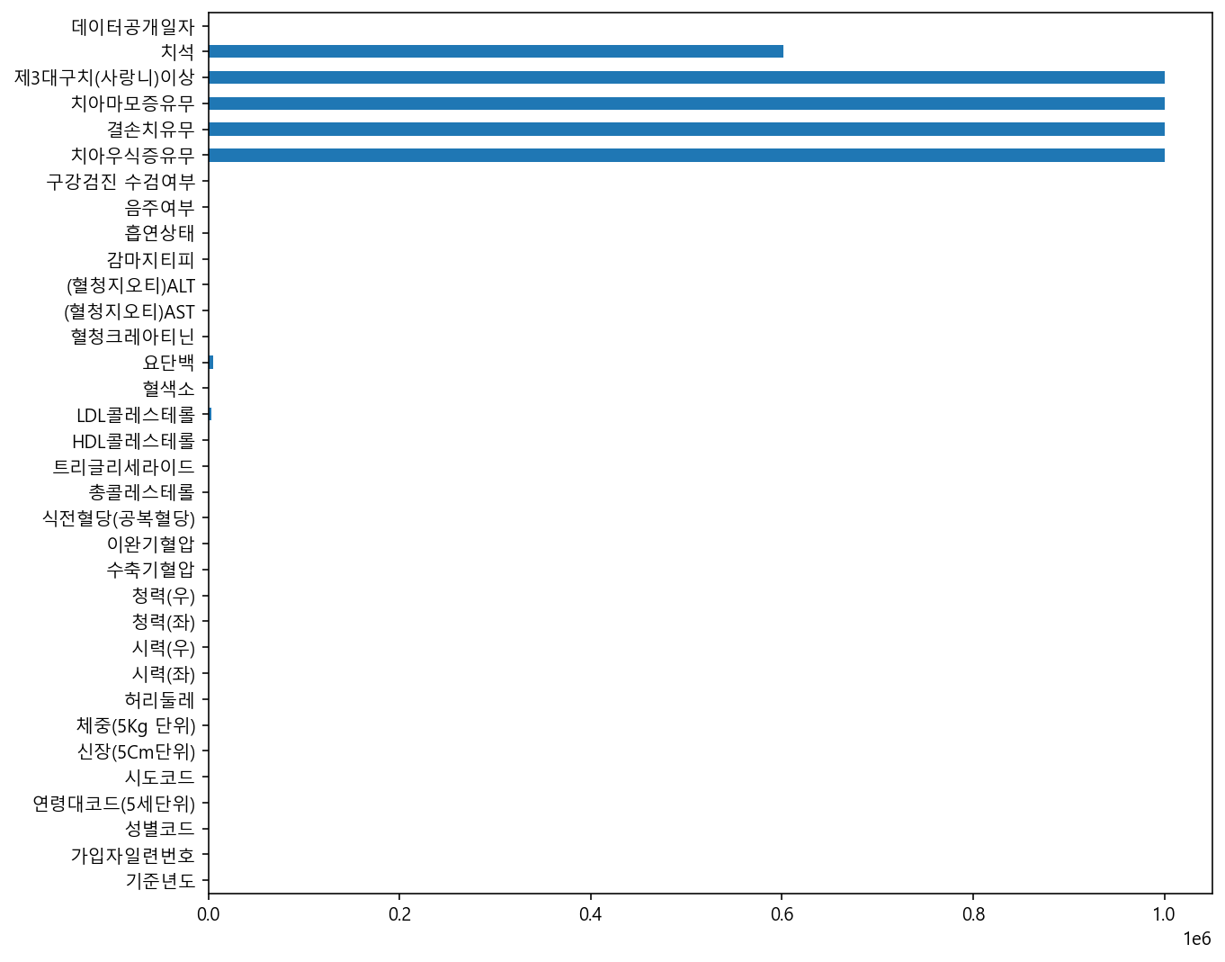
일부 데이터 요약하기
# 여러 컬럼을 가져온다.
# "(혈청지오티)ALT", "(혈청지오티)AST"를 가져와 미리보기 한다.
df["(혈청지오티)ALT", "(혈청지오티)AST"]

# 오류가 난다!! 두개 이상의 데이터를 불러 올 때는 리스트 자료 구조로 가져와야 한다.
KeyError: ('(혈청지오티)ALT', '(혈청지오티)AST')df[["(혈청지오티)ALT", "(혈청지오티)AST"]].head()| (혈청지오티)ALT | (혈청지오티)AST | |
|---|---|---|
| 0 | 41.0 | 19.0 |
| 1 | 13.0 | 16.0 |
| 2 | 62.0 | 45.0 |
| 3 | 24.0 | 21.0 |
| 4 | 62.0 | 37.0 |
# "(혈청지오티)ALT", "(혈청지오티)AST"를 요약
df[["(혈청지오티)ALT", "(혈청지오티)AST"]].info()
<class 'pandas.core.frame.DataFrame'>
RangeIndex: 1000000 entries, 0 to 999999
Data columns (total 2 columns):
# Column Non-Null Count Dtype
--- ------ -------------- -----
0 (혈청지오티)ALT 999956 non-null float64
1 (혈청지오티)AST 999958 non-null float64
dtypes: float64(2)
memory usage: 15.3 MBdf[["(혈청지오티)ALT", "(혈청지오티)AST"]].describe()| (혈청지오티)ALT | (혈청지오티)AST | |
|---|---|---|
| count | 999956.000000 | 999958.000000 |
| mean | 25.859343 | 26.075068 |
| std | 25.814268 | 24.437136 |
| min | 1.000000 | 1.000000 |
| 25% | 15.000000 | 19.000000 |
| 50% | 20.000000 | 23.000000 |
| 75% | 30.000000 | 28.000000 |
| max | 6710.000000 | 9999.000000 |
value_counts로 값 집계하기
# 성별코드로 그룹화 하고 갯수 집계하기
df["성별코드"].value_counts()
1 531172
2 468828
Name: 성별코드, dtype: int64# 흡연상태로 그룹화 하고 갯수 집계하기
df["흡연상태"].value_counts()
# 1:노흡연 3:흡연자 2:흡연했따가 금연1.0 608587
3.0 215061
2.0 176192
Name: 흡연상태, dtype: int64groupby와 pivot_table 사용
groupby
# 성별코드로 그룹화 한 데이터 세어보기
df.groupby?df.groupby(["성별코드"])["가입자일련번호"].count()성별코드
1 531172
2 468828
Name: 가입자일련번호, dtype: int64# 성별코드와 음주여부로 그룹화 하고 갯수 세기
df.groupby(["성별코드", "음주여부"])["가입자일련번호"].count()성별코드 음주여부
1 0.0 175150
1.0 355826
2 0.0 327579
1.0 140920
Name: 가입자일련번호, dtype: int64# 성별코드와 음주여부로 그룹화 하고 감마지티피의 평균 구하기
df.groupby(["성별코드", "음주여부"])["감마지티피"].mean()성별코드 음주여부
1 0.0 34.710544
1.0 56.707919
2 0.0 22.660238
1.0 25.115149
Name: 감마지티피, dtype: float64# 성별코드와 음주여부로 그룹화를 하고 감마지티피의 요약수치를 구한다.
df.groupby(["성별코드", "음주여부"])["감마지티피"].describe()| count | mean | std | min | 25% | 50% | 75% | max | ||
|---|---|---|---|---|---|---|---|---|---|
| 성별코드 | 음주여부 | ||||||||
| 1 | 0.0 | 175139.0 | 34.710544 | 37.715218 | 1.0 | 18.0 | 25.0 | 38.0 | 999.0 |
| 1.0 | 355819.0 | 56.707919 | 69.039084 | 1.0 | 24.0 | 37.0 | 63.0 | 999.0 | |
| 2 | 0.0 | 327559.0 | 22.660238 | 25.181300 | 1.0 | 13.0 | 17.0 | 24.0 | 999.0 |
| 1.0 | 140913.0 | 25.115149 | 35.870812 | 1.0 | 13.0 | 17.0 | 25.0 | 999.0 |
# agg를 사용하면 여러 수치를 함께 구할 수 있다.
df.groupby(["성별코드", "음주여부"])["감마지티피"].agg(["count","mean","median"])| count | mean | median | ||
|---|---|---|---|---|
| 성별코드 | 음주여부 | |||
| 1 | 0.0 | 175139 | 34.710544 | 25.0 |
| 1.0 | 355819 | 56.707919 | 37.0 | |
| 2 | 0.0 | 327559 | 22.660238 | 17.0 |
| 1.0 | 140913 | 25.115149 | 17.0 |
pivot_table
# 음주여부에 따른 그룹화된 수 피봇테이블 구하기
df.pivot_table(index="음주여부")| (혈청지오티)ALT | (혈청지오티)AST | HDL콜레스테롤 | LDL콜레스테롤 | 가입자일련번호 | 감마지티피 | 구강검진 수검여부 | 기준년도 | 데이터공개일자 | 성별코드 | ... | 청력(우) | 청력(좌) | 체중(5Kg 단위) | 총콜레스테롤 | 치석 | 트리글리세라이드 | 허리둘레 | 혈색소 | 혈청크레아티닌 | 흡연상태 | |
|---|---|---|---|---|---|---|---|---|---|---|---|---|---|---|---|---|---|---|---|---|---|
| 음주여부 | |||||||||||||||||||||
| 0.0 | 24.107862 | 25.094792 | 56.161852 | 114.467632 | 499800.113284 | 26.858541 | 0.358768 | 2017 | 20181126 | 1.651602 | ... | 1.041086 | 1.042881 | 60.082827 | 194.699007 | 0.573111 | 122.063887 | 80.269019 | 13.748950 | 0.837132 | 1.320330 |
| 1.0 | 27.634991 | 27.069879 | 57.606351 | 111.444394 | 500196.825986 | 47.745678 | 0.439257 | 2017 | 20181126 | 1.283686 | ... | 1.020745 | 1.021758 | 66.778226 | 196.346568 | 0.626153 | 144.077696 | 82.484576 | 14.704997 | 0.892460 | 1.896158 |
2 rows × 29 columns
df.pivot_table(index="음주여부", values="가입자일련번호", aggfunc="count")
# mean값이 기본 세팅값이므로 aggfunc로 바꿔주기. | 가입자일련번호 | |
|---|---|
| 음주여부 | |
| 0.0 | 502729 |
| 1.0 | 496746 |
df.pivot_table(index="성별코드", values="가입자일련번호", aggfunc="count")
# data frame으로 출력된다! | 가입자일련번호 | |
|---|---|
| 성별코드 | |
| 1 | 531172 |
| 2 | 468828 |
# 음주여부에 따른 감마지티피의 평균 구하기

pd.pivot_table(df, index="음주여부", values="감마지티피")| 감마지티피 | |
|---|---|
| 음주여부 | |
| 0.0 | 26.858541 |
| 1.0 | 47.745678 |
# 기본값은 평균을 구하지만 aggfunc를 통해 지정이 가능하다.

pd.pivot_table(df, index="음주여부", values="감마지티피", aggfunc=["mean", "median"])| mean | median | |
|---|---|---|
| 감마지티피 | 감마지티피 | |
| 음주여부 | ||
| 0.0 | 26.858541 | 19.0 |
| 1.0 | 47.745678 | 30.0 |
# aggfunc에 describe를 사용해 통계요약값을 볼수있다.

pd.pivot_table(df, index=["성별코드", "음주여부"], values="감마지티피", aggfunc="describe")| 25% | 50% | 75% | count | max | mean | min | std | ||
|---|---|---|---|---|---|---|---|---|---|
| 성별코드 | 음주여부 | ||||||||
| 1 | 0.0 | 18.0 | 25.0 | 38.0 | 175139.0 | 999.0 | 34.710544 | 1.0 | 37.715218 |
| 1.0 | 24.0 | 37.0 | 63.0 | 355819.0 | 999.0 | 56.707919 | 1.0 | 69.039084 | |
| 2 | 0.0 | 13.0 | 17.0 | 24.0 | 327559.0 | 999.0 | 22.660238 | 1.0 | 25.181300 |
| 1.0 | 13.0 | 17.0 | 25.0 | 140913.0 | 999.0 | 25.115149 | 1.0 | 35.870812 |
전체 데이터 시각화 하기
100만개가 넘는 데이터를 시각화할 때는 시각화하는 속도가 느리기 때문에 groupby 또는 pivot_table로 연산을 하여 시각화하거나 필요한 데이터만 추출해서 시각화해보시길 권장합니다.
메모리 용량을 줄이기 위해서 대부분의 수치 데이터로 이루어져 있습니다.
히스토그램
df.hist(figsize=(12,12))array([[<AxesSubplot:title={'center':'기준년도'}>,
<AxesSubplot:title={'center':'가입자일련번호'}>,
<AxesSubplot:title={'center':'성별코드'}>,
<AxesSubplot:title={'center':'연령대코드(5세단위)'}>,
<AxesSubplot:title={'center':'시도코드'}>,
<AxesSubplot:title={'center':'신장(5Cm단위)'}>],
[<AxesSubplot:title={'center':'체중(5Kg 단위)'}>,
<AxesSubplot:title={'center':'허리둘레'}>,
<AxesSubplot:title={'center':'시력(좌)'}>,
<AxesSubplot:title={'center':'시력(우)'}>,
<AxesSubplot:title={'center':'청력(좌)'}>,
<AxesSubplot:title={'center':'청력(우)'}>],
[<AxesSubplot:title={'center':'수축기혈압'}>,
<AxesSubplot:title={'center':'이완기혈압'}>,
<AxesSubplot:title={'center':'식전혈당(공복혈당)'}>,
<AxesSubplot:title={'center':'총콜레스테롤'}>,
<AxesSubplot:title={'center':'트리글리세라이드'}>,
<AxesSubplot:title={'center':'HDL콜레스테롤'}>],
[<AxesSubplot:title={'center':'LDL콜레스테롤'}>,
<AxesSubplot:title={'center':'혈색소'}>,
<AxesSubplot:title={'center':'요단백'}>,
<AxesSubplot:title={'center':'혈청크레아티닌'}>,
<AxesSubplot:title={'center':'(혈청지오티)AST'}>,
<AxesSubplot:title={'center':'(혈청지오티)ALT'}>],
[<AxesSubplot:title={'center':'감마지티피'}>,
<AxesSubplot:title={'center':'흡연상태'}>,
<AxesSubplot:title={'center':'음주여부'}>,
<AxesSubplot:title={'center':'구강검진 수검여부'}>,
<AxesSubplot:title={'center':'치아우식증유무'}>,
<AxesSubplot:title={'center':'결손치유무'}>],
[<AxesSubplot:title={'center':'치아마모증유무'}>,
<AxesSubplot:title={'center':'제3대구치(사랑니)이상'}>,
<AxesSubplot:title={'center':'치석'}>,
<AxesSubplot:title={'center':'데이터공개일자'}>, <AxesSubplot:>,
<AxesSubplot:>]], dtype=object)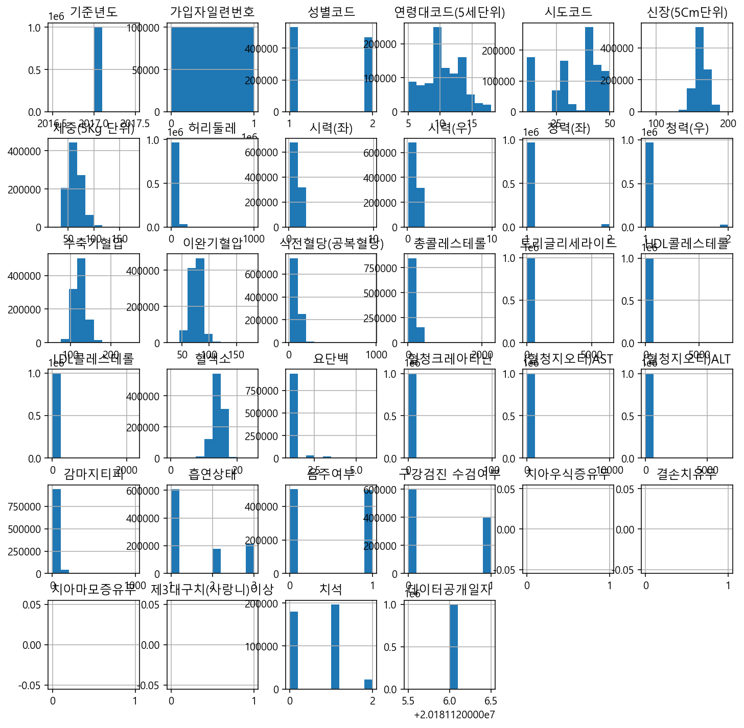
h = df.hist(figsize=(12,12)) 
슬라이싱을 사용해 히스토그램 그래기
# [행, 열]
df.iloc[:,:] # 몇번째에 있는 행인지, 컬럼인지 지정 가능
# [:,:] 전체데이터| 기준년도 | 가입자일련번호 | 성별코드 | 연령대코드(5세단위) | 시도코드 | 신장(5Cm단위) | 체중(5Kg 단위) | 허리둘레 | 시력(좌) | 시력(우) | ... | 감마지티피 | 흡연상태 | 음주여부 | 구강검진 수검여부 | 치아우식증유무 | 결손치유무 | 치아마모증유무 | 제3대구치(사랑니)이상 | 치석 | 데이터공개일자 | |
|---|---|---|---|---|---|---|---|---|---|---|---|---|---|---|---|---|---|---|---|---|---|
| 0 | 2017 | 1 | 1 | 13 | 46 | 170.0 | 65.0 | 91.0 | 1.0 | 1.2 | ... | 25.0 | 3.0 | 0.0 | 1 | NaN | NaN | NaN | NaN | 1.0 | 20181126 |
| 1 | 2017 | 2 | 2 | 8 | 41 | 150.0 | 45.0 | 73.4 | 1.2 | 1.0 | ... | 10.0 | 1.0 | 0.0 | 1 | NaN | NaN | NaN | NaN | 1.0 | 20181126 |
| 2 | 2017 | 3 | 1 | 8 | 45 | 175.0 | 75.0 | 94.0 | 1.0 | 0.8 | ... | 136.0 | 1.0 | 0.0 | 1 | NaN | NaN | NaN | NaN | 0.0 | 20181126 |
| 3 | 2017 | 4 | 2 | 12 | 11 | 155.0 | 55.0 | 67.5 | 0.9 | 1.0 | ... | 30.0 | 1.0 | 1.0 | 0 | NaN | NaN | NaN | NaN | NaN | 20181126 |
| 4 | 2017 | 5 | 1 | 8 | 41 | 175.0 | 75.0 | 93.0 | 1.5 | 1.5 | ... | 68.0 | 3.0 | 0.0 | 0 | NaN | NaN | NaN | NaN | NaN | 20181126 |
| ... | ... | ... | ... | ... | ... | ... | ... | ... | ... | ... | ... | ... | ... | ... | ... | ... | ... | ... | ... | ... | ... |
| 999995 | 2017 | 999996 | 2 | 9 | 41 | 165.0 | 55.0 | 70.0 | 1.5 | 1.5 | ... | 11.0 | 1.0 | 1.0 | 0 | NaN | NaN | NaN | NaN | NaN | 20181126 |
| 999996 | 2017 | 999997 | 2 | 9 | 11 | 165.0 | 50.0 | 68.0 | 1.2 | 1.5 | ... | 11.0 | 1.0 | 0.0 | 1 | NaN | NaN | NaN | NaN | 0.0 | 20181126 |
| 999997 | 2017 | 999998 | 2 | 12 | 27 | 155.0 | 50.0 | 83.8 | 0.2 | 1.0 | ... | 12.0 | 1.0 | 0.0 | 1 | NaN | NaN | NaN | NaN | 0.0 | 20181126 |
| 999998 | 2017 | 999999 | 1 | 11 | 47 | 160.0 | 70.0 | 99.0 | 0.8 | 0.9 | ... | 35.0 | 2.0 | 1.0 | 0 | NaN | NaN | NaN | NaN | NaN | 20181126 |
| 999999 | 2017 | 1000000 | 2 | 9 | 27 | 165.0 | 60.0 | 74.0 | 1.2 | 1.2 | ... | 15.0 | 1.0 | 0.0 | 0 | NaN | NaN | NaN | NaN | NaN | 20181126 |
1000000 rows × 34 columns
df.iloc[:,:12].hist(figsize=(12,12))array([[<AxesSubplot:title={'center':'기준년도'}>,
<AxesSubplot:title={'center':'가입자일련번호'}>,
<AxesSubplot:title={'center':'성별코드'}>],
[<AxesSubplot:title={'center':'연령대코드(5세단위)'}>,
<AxesSubplot:title={'center':'시도코드'}>,
<AxesSubplot:title={'center':'신장(5Cm단위)'}>],
[<AxesSubplot:title={'center':'체중(5Kg 단위)'}>,
<AxesSubplot:title={'center':'허리둘레'}>,
<AxesSubplot:title={'center':'시력(좌)'}>],
[<AxesSubplot:title={'center':'시력(우)'}>,
<AxesSubplot:title={'center':'청력(좌)'}>,
<AxesSubplot:title={'center':'청력(우)'}>]], dtype=object)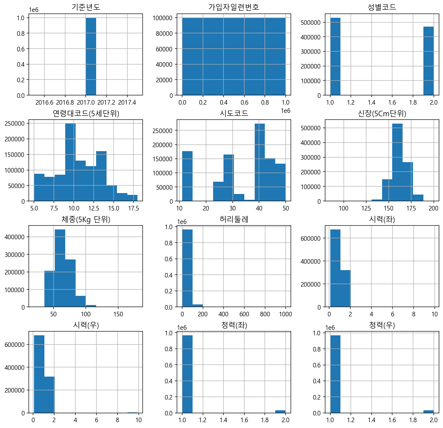
# 슬라이싱을 사용해 앞에서 12번째부터 23번쨰까지 (12:24)
h = df.iloc[:,12:24].hist(figsize=(12,12), bins=100)   # bins : 막대 개수를 더 ...  연속된 수치데이터를 카테고리 형태로!!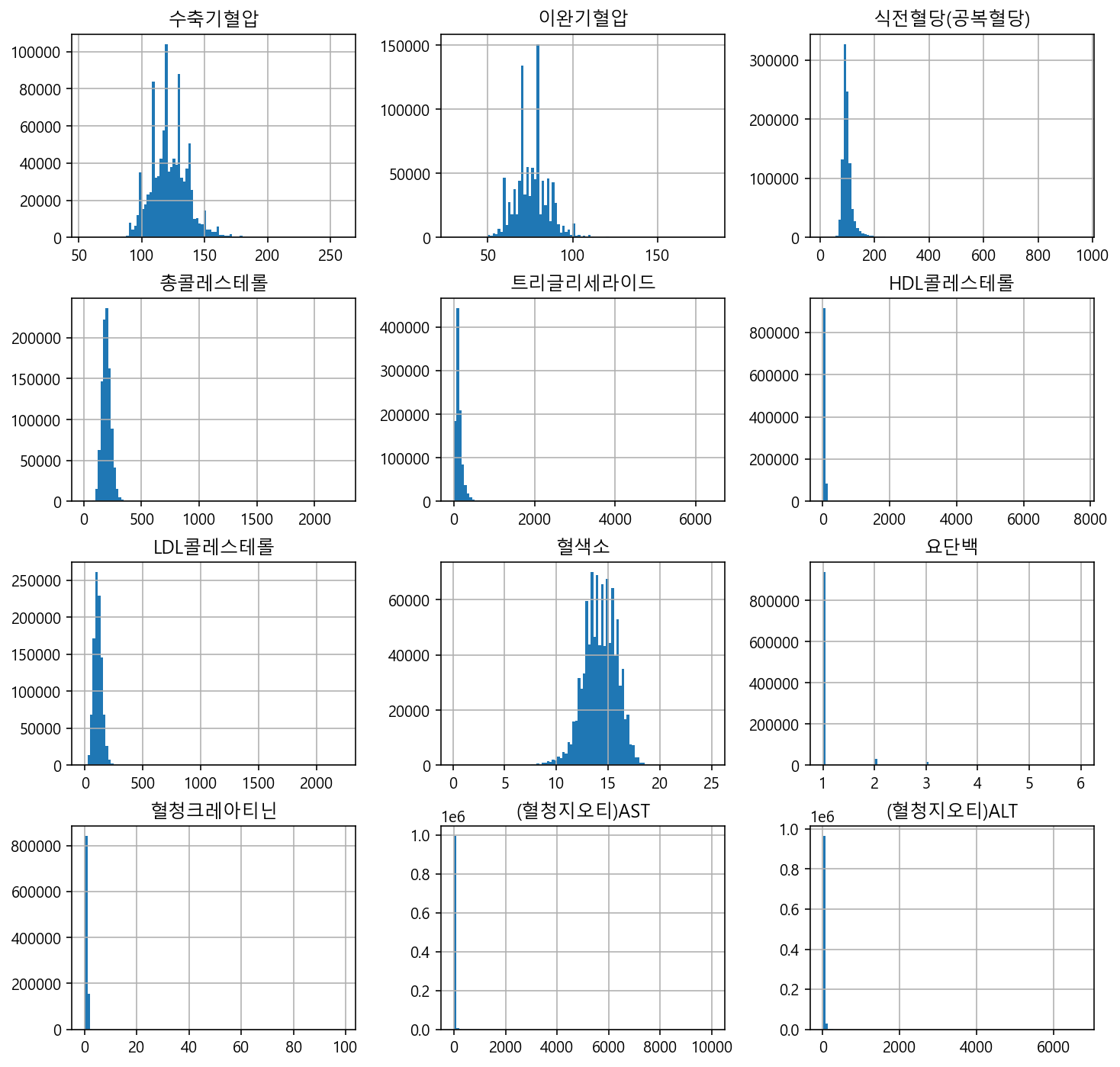
샘플데이터 추출하기
- seaborn의 그래프는 내부에서 수학적 연산이 되어 데이터가 많으면 속도가 오래걸린다.
df.sample()| 기준년도 | 가입자일련번호 | 성별코드 | 연령대코드(5세단위) | 시도코드 | 신장(5Cm단위) | 체중(5Kg 단위) | 허리둘레 | 시력(좌) | 시력(우) | ... | 감마지티피 | 흡연상태 | 음주여부 | 구강검진 수검여부 | 치아우식증유무 | 결손치유무 | 치아마모증유무 | 제3대구치(사랑니)이상 | 치석 | 데이터공개일자 | |
|---|---|---|---|---|---|---|---|---|---|---|---|---|---|---|---|---|---|---|---|---|---|
| 876744 | 2017 | 876745 | 2 | 13 | 47 | 150.0 | 55.0 | 72.0 | 0.7 | 0.5 | ... | 29.0 | 1.0 | 0.0 | 0 | NaN | NaN | NaN | NaN | NaN | 20181126 |
1 rows × 34 columns
df_sample = df.sample(1000,random_state=1) #random_state : 항상 같은 값을 반환한다. dfdf_sample.shape(1000, 34)데이터 시각화 도구 seaborn 사용하기
- https://seaborn.pydata.org/
- seaborn은 https://matplotilb.org/ 사용하기 쉽게 만들어 졌고, 간단하게 고급 통계 연산을 할 수 있다.
범주형(카테고리) 데이터 시각화
- countplot은 범주형 데이터의 수를 더한 값을 그래프로 표현
- value_counts 로 구한 값을 시각화
countplot - 음주여부
# 음주여부에 따른 countplot을 그린다
df["음주여부"].value_counts().plot.bar()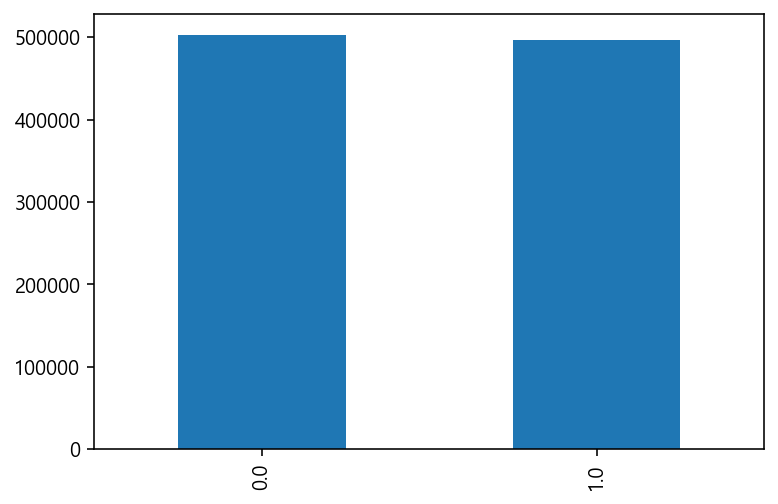
sns.countplot(x="음주여부", data=df)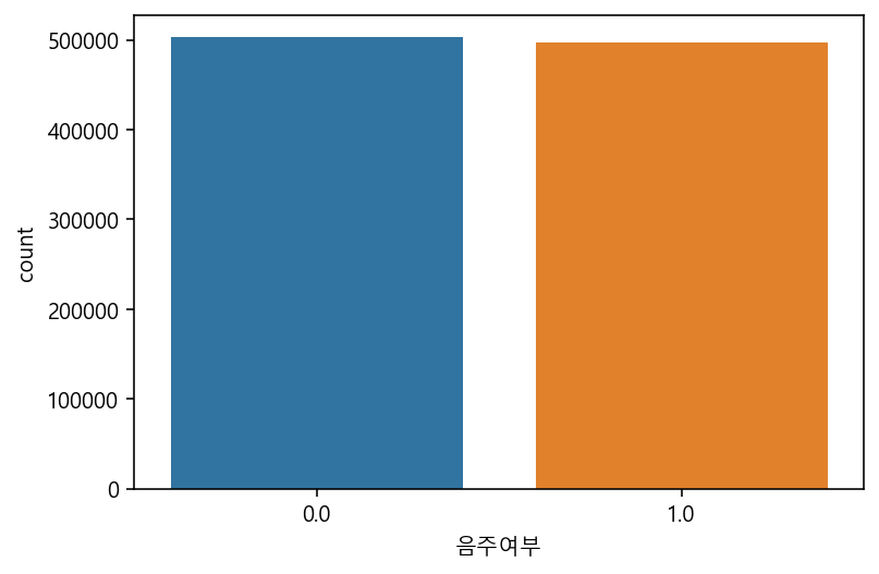
sns.countplot(x="흡연상태", data=df)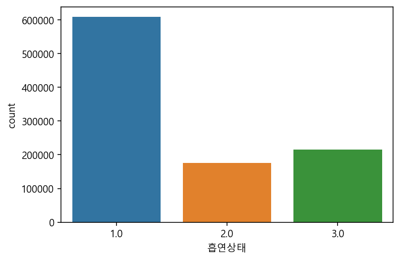
hue 옵션 사용하기
#window
# sns.set(font_scale=1.5, font="Malgun Gothic") 이렇게도 사용 가능

sns.countplot(data=df, x="음주여부", hue="성별코드")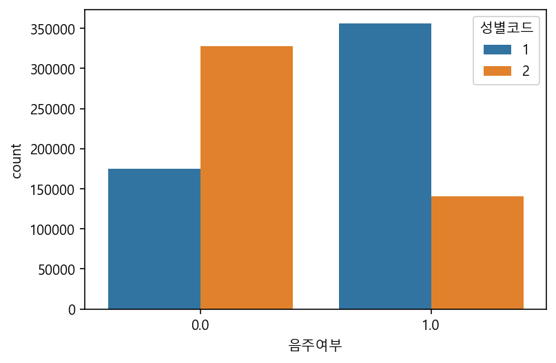
sns.countplot(data=df, x="연령대코드(5세단위)", hue="음주여부") 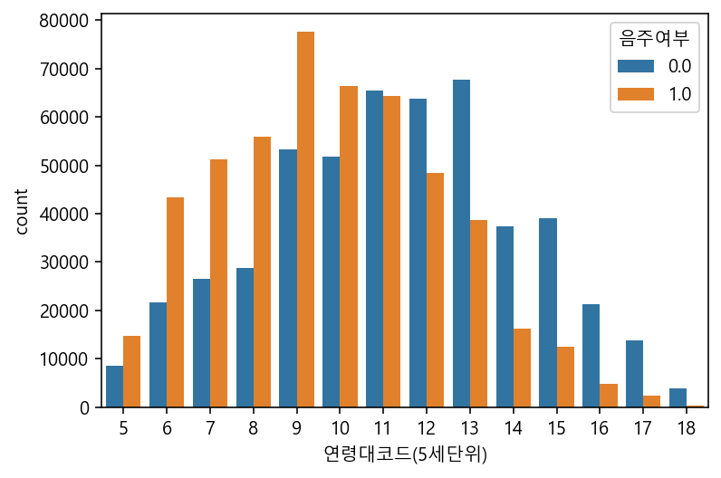
countplot - 키와 몸무게
- 키와 몸무게는 연속형 데이터이다.
- 하지만 데이터는 키는 5cm, 체중은 5kg 단위로 되어 있다.
- 이렇게 특정 범위로 묶게 되면 연속형 데이터라기 보다는 범주형 데이터라고 본다.
plt.figure(figsize=(15,4))
sns.countplot(data=df, x="신장(5Cm단위)")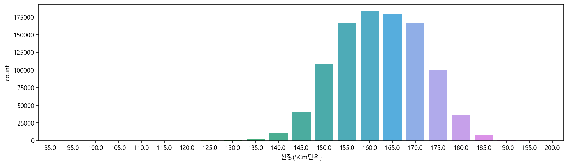
plt.figure(figsize=(15,4))
sns.countplot(data=df, x="체중(5Kg 단위)")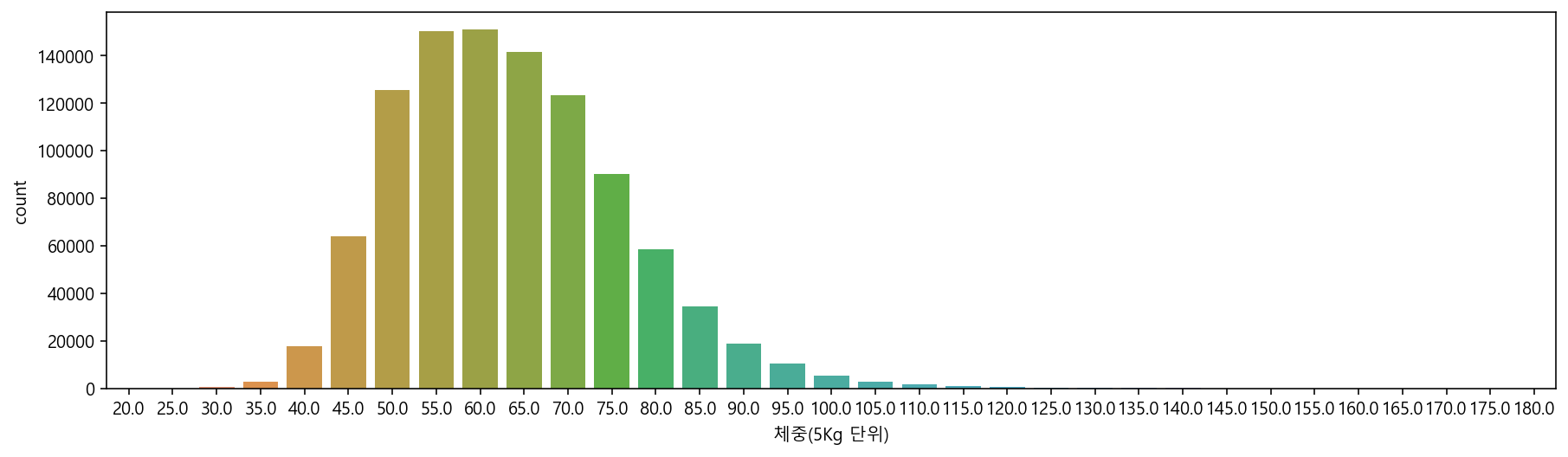
plt.figure(figsize=(15,4))
sns.countplot(data=df, x="신장(5Cm단위)", hue="성별코드")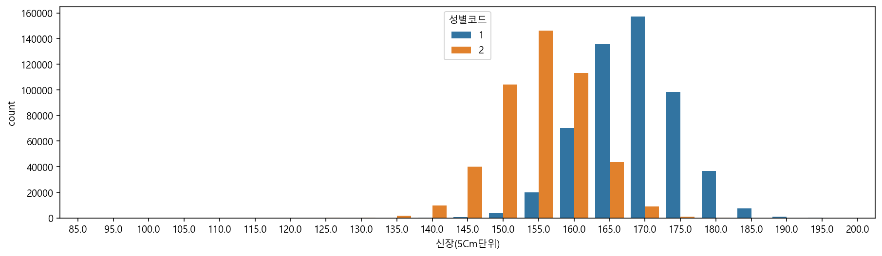
plt.figure(figsize=(15,4))
sns.countplot(data=df, x="체중(5Kg 단위)", hue="성별코드")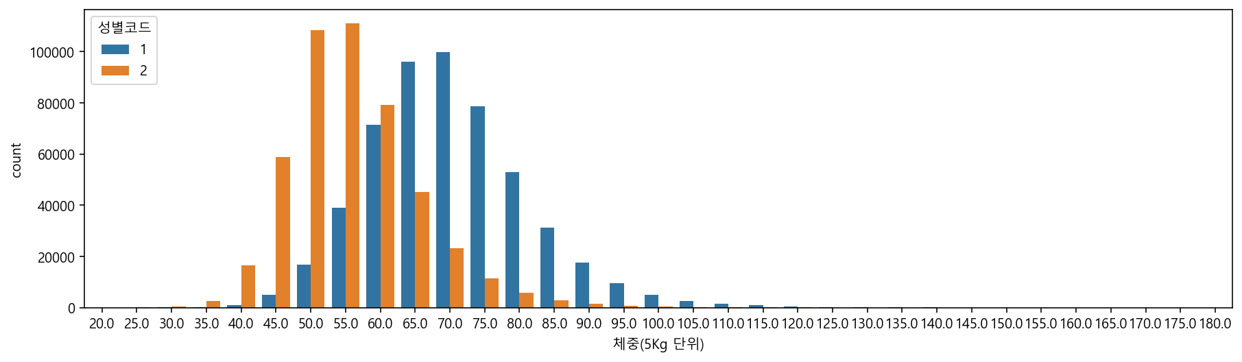
plt.figure(figsize=(15,4))
sns.countplot(data=df, x="체중(5Kg 단위)", hue="음주여부")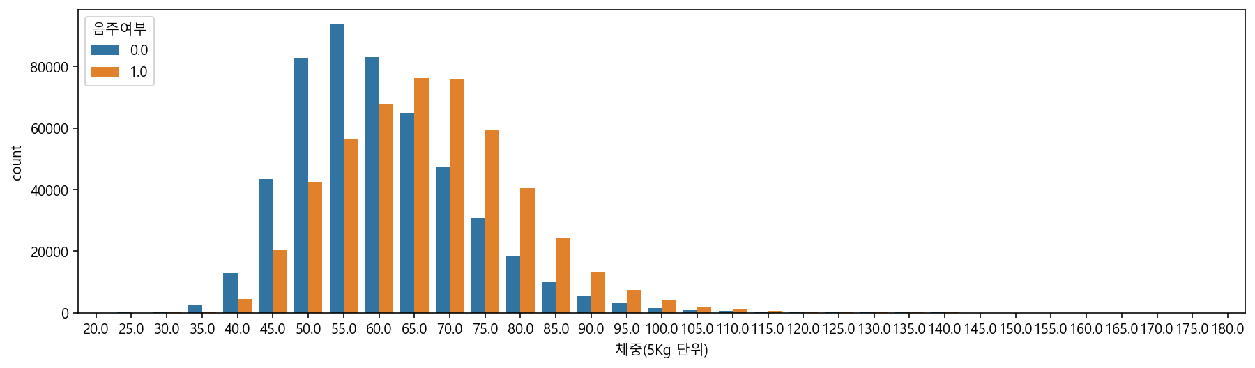
14. 4 braplot - 수치형 vs 범주형
# 연령대코드와 총 콜레스테롤 보기
# hue로 색상 다르게 표현. 음주여부 같이 보기

sns.barplot(data=df, x="연령대코드(5세단위)", y="총콜레스테롤", hue="음주여부")

# 느리다! countplot와 비교했을때 ! 백만개의 데이터가 있는데.. 연령대 코드별로 총 콜레스테롤을 그리긴 했지만. .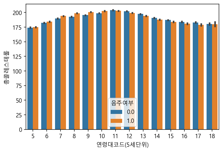
plt.figure(figsize=(15,4))
sns.barplot(data=df, x="연령대코드(5세단위)", y="총콜레스테롤", hue="흡연상태")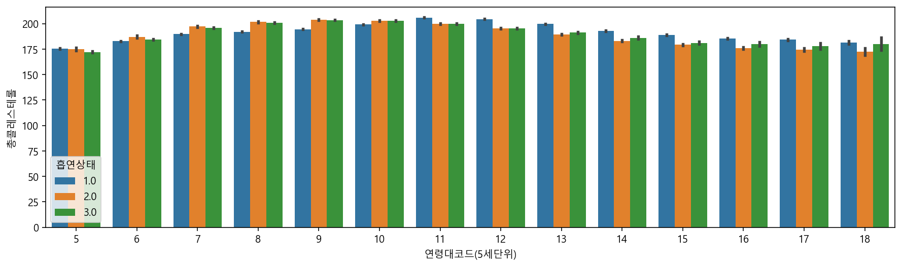
plt.figure(figsize=(15,4))
sns.barplot(data=df_sample, x="연령대코드(5세단위)", y="총콜레스테롤", hue="흡연상태")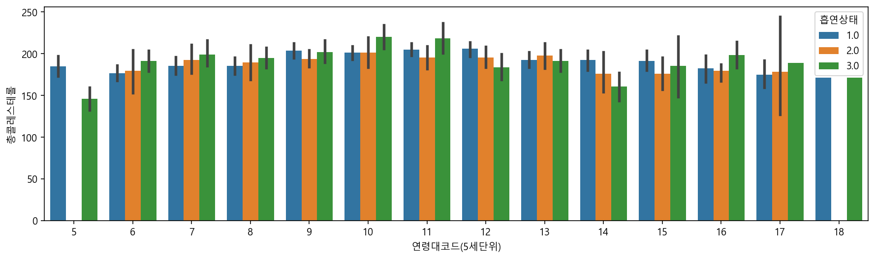
#트리글리세라이드(중성지방)에 따른 연령대코드(5세단위)를 음주여부에 따라 barplot로 그리기
sns.barplot(data=df_sample, x="연령대코드(5세단위)", y="트리글리세라이드", hue="음주여부", ci=95)

# 검은색 막대: 신뢰구간을 의미 (ci: 95)-> 95%의 신뢰구간을 표시한다.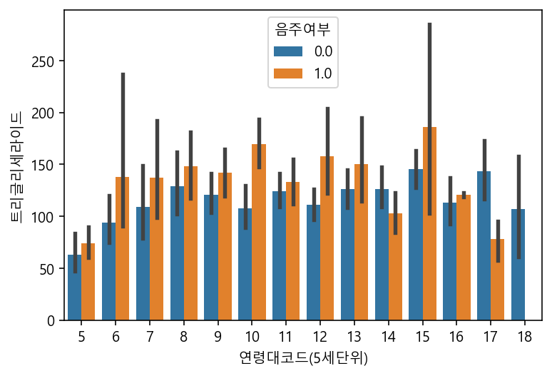
sns.barplot(data=df_sample, x="연령대코드(5세단위)", y="트리글리세라이드", hue="음주여부", ci="sd") #sd:표준편차
# sample로 그려서 편차가 커보인다. 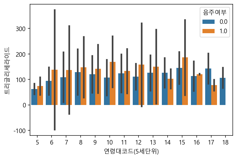
sns.barplot(data=df, x="연령대코드(5세단위)", y="트리글리세라이드", hue="음주여부", ci="sd") #sd:표준편차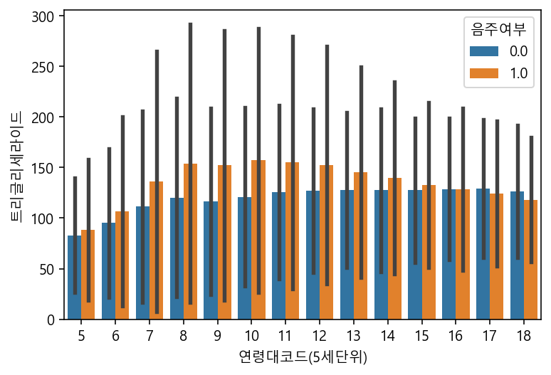
sns.barplot(data=df, x="연령대코드(5세단위)", y="트리글리세라이드", hue="음주여부", ci=None) #sd:표준편차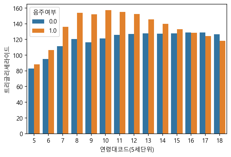
# 연령대코드와 체중(5kg 단위)을 성별에 따라서.
sns.barplot(data=df, x="연령대코드(5세단위)", y="체중(5Kg 단위)", hue="성별코드", ci=None) 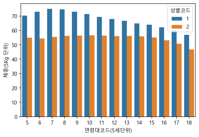
sns.barplot(data=df, x="연령대코드(5세단위)", y="체중(5Kg 단위)", hue="음주여부", ci=None)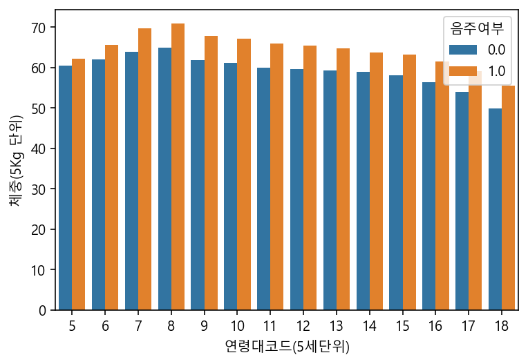
lineplot and pointplot
sns.lineplot(data=df, x="연령대코드(5세단위)", y="체중(5Kg 단위)", hue="성별코드", ci=None)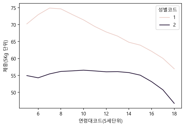
sns.lineplot(data=df_sample, x="연령대코드(5세단위)", y="체중(5Kg 단위)", hue="성별코드")
# 그림자로 표시!! 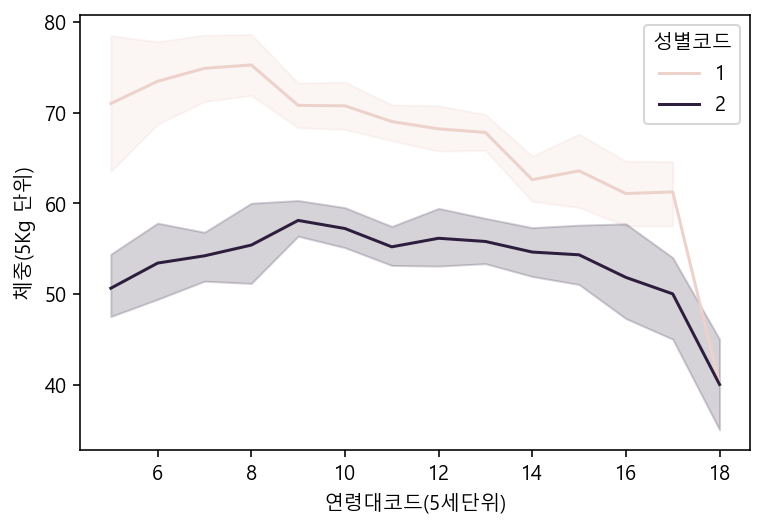
plt.figure(figsize=(15,4))
sns.lineplot(data=df_sample, x="연령대코드(5세단위)", y="체중(5Kg 단위)", hue="성별코드", ci="sd")
# 그림자로 표시!! 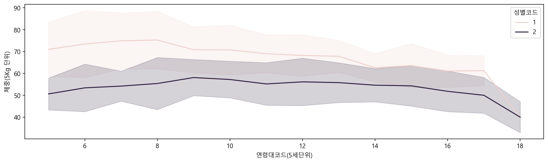
plt.figure(figsize=(15,4))
sns.lineplot(data=df_sample, x="연령대코드(5세단위)", y="신장(5Cm단위)", hue="성별코드", ci="sd")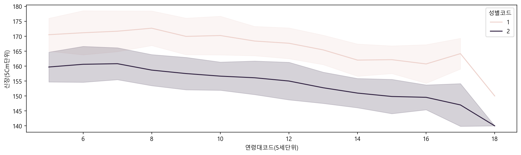
plt.figure(figsize=(15,4))
sns.lineplot(data=df_sample, x="연령대코드(5세단위)", y="신장(5Cm단위)", hue="음주여부", ci="sd")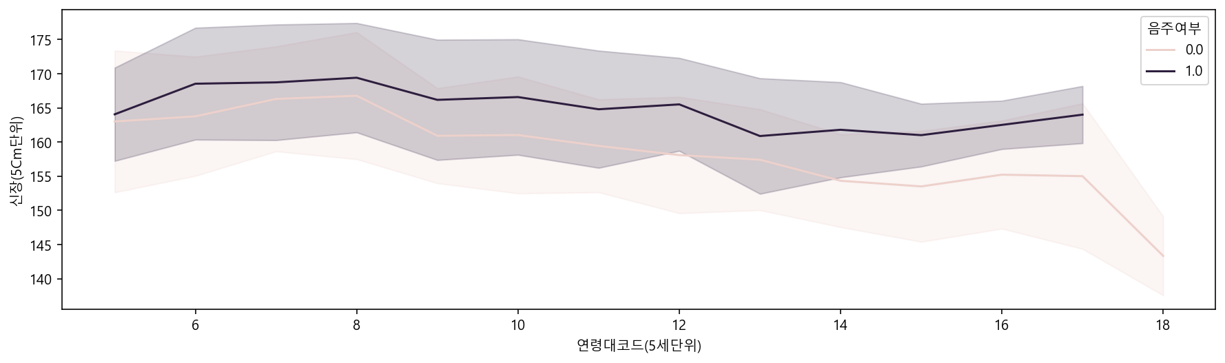
plt.figure(figsize=(15,4))
sns.pointplot(data=df_sample, x="연령대코드(5세단위)", y="신장(5Cm단위)", hue="음주여부", ci="sd")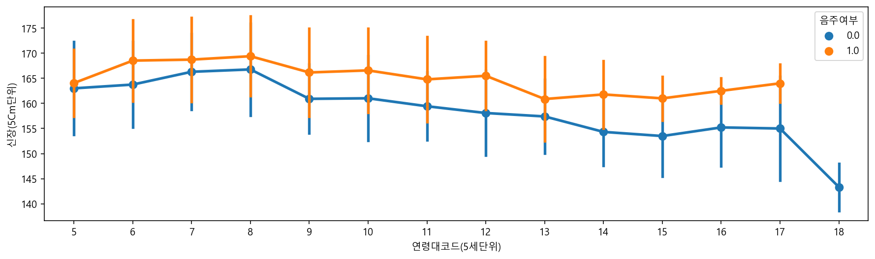
plt.figure(figsize=(15,4))
sns.barplot(data=df_sample, x="연령대코드(5세단위)", y="신장(5Cm단위)", hue="음주여부", ci="sd")
sns.pointplot(data=df_sample, x="연령대코드(5세단위)", y="신장(5Cm단위)", hue="음주여부", ci="sd")
# 두개를 겹쳐서 그릴 수도 있다.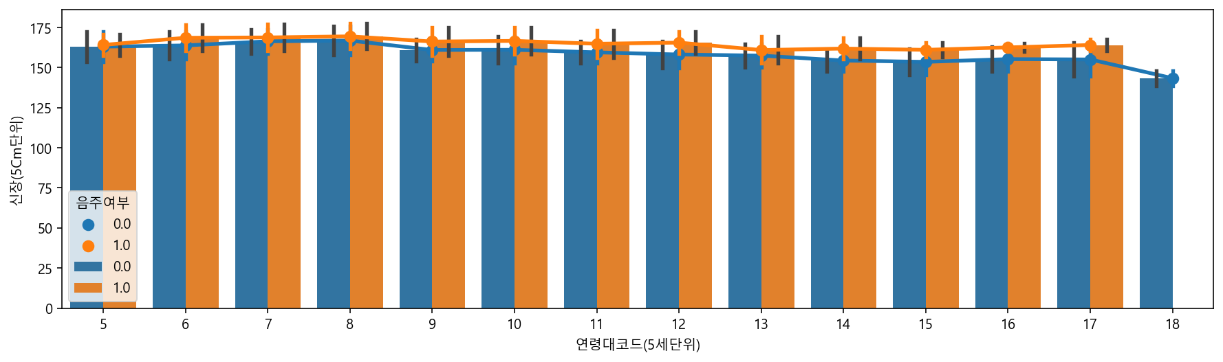
plt.figure(figsize=(15,4))
sns.lineplot(data=df, x="연령대코드(5세단위)", y="혈색소", hue="음주여부", ci=None)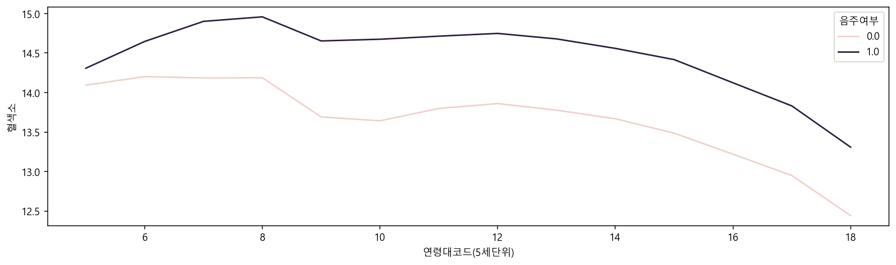
boxplot
# boxplot으로 신장에 따른 체중을 그리며, 성별코드에 따른 색상으로 표현하기
plt.figure(figsize=(15,4))
sns.boxplot(data=df, x="신장(5Cm단위)", y="체중(5Kg 단위)", hue="성별코드")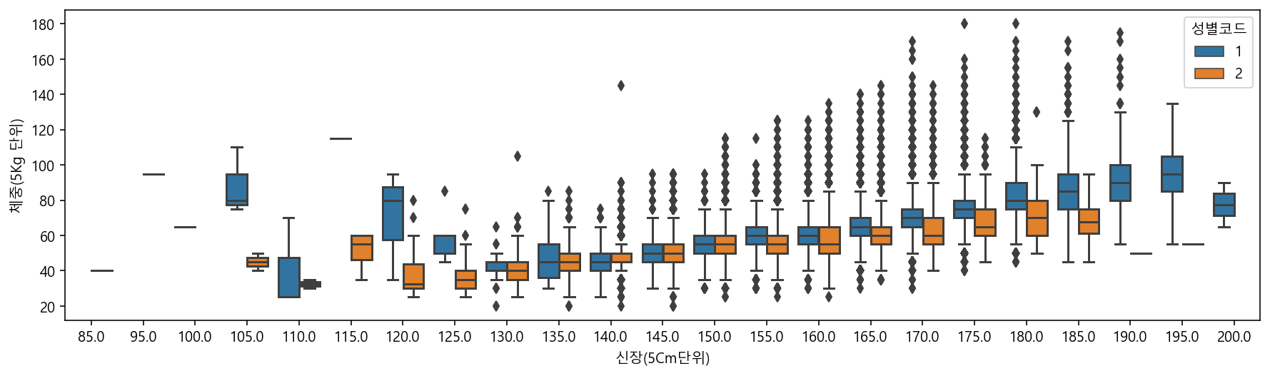
plt.figure(figsize=(15,4))
sns.boxplot(data=df, x="신장(5Cm단위)", y="체중(5Kg 단위)", hue="음주여부")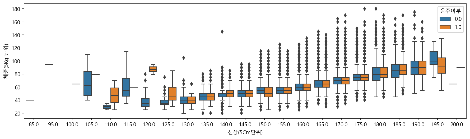
violinplot
plt.figure(figsize=(15,4))
sns.violinplot(data=df, x="신장(5Cm단위)", y="체중(5Kg 단위)")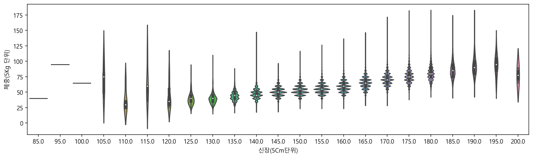
plt.figure(figsize=(15,4))
sns.violinplot(data=df_sample, x="신장(5Cm단위)", y="체중(5Kg 단위)", hue="음주여부")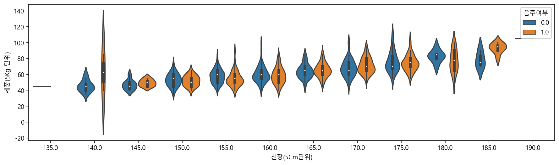
plt.figure(figsize=(15,4))
sns.violinplot(data=df_sample, x="신장(5Cm단위)", y="체중(5Kg 단위)", hue="음주여부", split=True)
# split : 두개의 값을 합쳐서 그림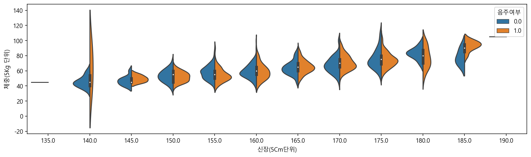
plt.figure(figsize=(15,4))
sns.violinplot(data=df_sample, x="연령대코드(5세단위)", y="혈색소", hue="음주여부", split=True)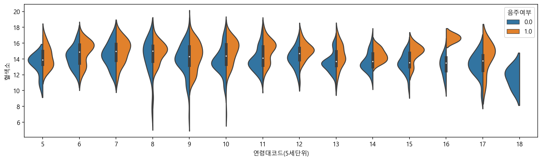
swarm plot
- 범주형 데이터를 산점도로 시각화하고자 할 대 사용한다.
plt.figure(figsize=(15,4))
sns.swarmplot(data=df_sample, x="신장(5Cm단위)", y="체중(5Kg 단위)", hue="음주여부")
C:\Users\user\anaconda3\lib\site-packages\seaborn\categorical.py:1296: UserWarning: 37.0% of the points cannot be placed; you may want to decrease the size of the markers or use stripplot.
warnings.warn(msg, UserWarning)
C:\Users\user\anaconda3\lib\site-packages\seaborn\categorical.py:1296: UserWarning: 52.7% of the points cannot be placed; you may want to decrease the size of the markers or use stripplot.
warnings.warn(msg, UserWarning)
C:\Users\user\anaconda3\lib\site-packages\seaborn\categorical.py:1296: UserWarning: 51.9% of the points cannot be placed; you may want to decrease the size of the markers or use stripplot.
warnings.warn(msg, UserWarning)
C:\Users\user\anaconda3\lib\site-packages\seaborn\categorical.py:1296: UserWarning: 55.4% of the points cannot be placed; you may want to decrease the size of the markers or use stripplot.
warnings.warn(msg, UserWarning)
C:\Users\user\anaconda3\lib\site-packages\seaborn\categorical.py:1296: UserWarning: 48.0% of the points cannot be placed; you may want to decrease the size of the markers or use stripplot.
warnings.warn(msg, UserWarning)
C:\Users\user\anaconda3\lib\site-packages\seaborn\categorical.py:1296: UserWarning: 26.0% of the points cannot be placed; you may want to decrease the size of the markers or use stripplot.
warnings.warn(msg, UserWarning)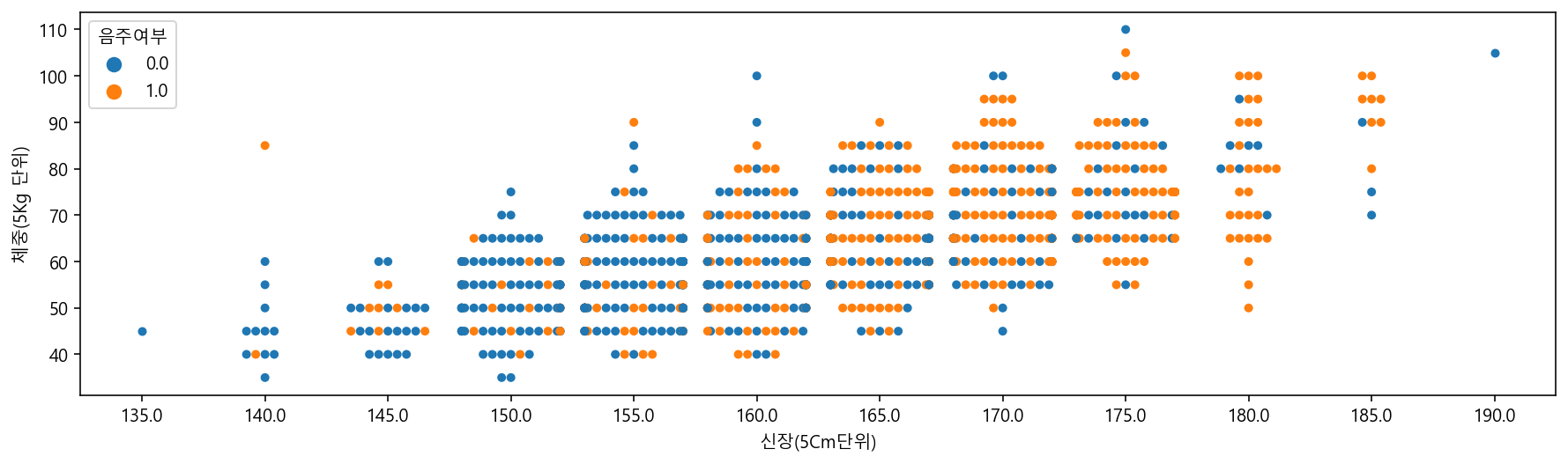
plt.figure(figsize=(15,4))
sns.swarmplot(data=df_sample, x="연령대코드(5세단위)", y="혈색소", hue="음주여부")
C:\Users\user\anaconda3\lib\site-packages\seaborn\categorical.py:1296: UserWarning: 7.1% of the points cannot be placed; you may want to decrease the size of the markers or use stripplot.
warnings.warn(msg, UserWarning)
C:\Users\user\anaconda3\lib\site-packages\seaborn\categorical.py:1296: UserWarning: 12.8% of the points cannot be placed; you may want to decrease the size of the markers or use stripplot.
warnings.warn(msg, UserWarning)
C:\Users\user\anaconda3\lib\site-packages\seaborn\categorical.py:1296: UserWarning: 9.3% of the points cannot be placed; you may want to decrease the size of the markers or use stripplot.
warnings.warn(msg, UserWarning)
C:\Users\user\anaconda3\lib\site-packages\seaborn\categorical.py:1296: UserWarning: 11.2% of the points cannot be placed; you may want to decrease the size of the markers or use stripplot.
warnings.warn(msg, UserWarning)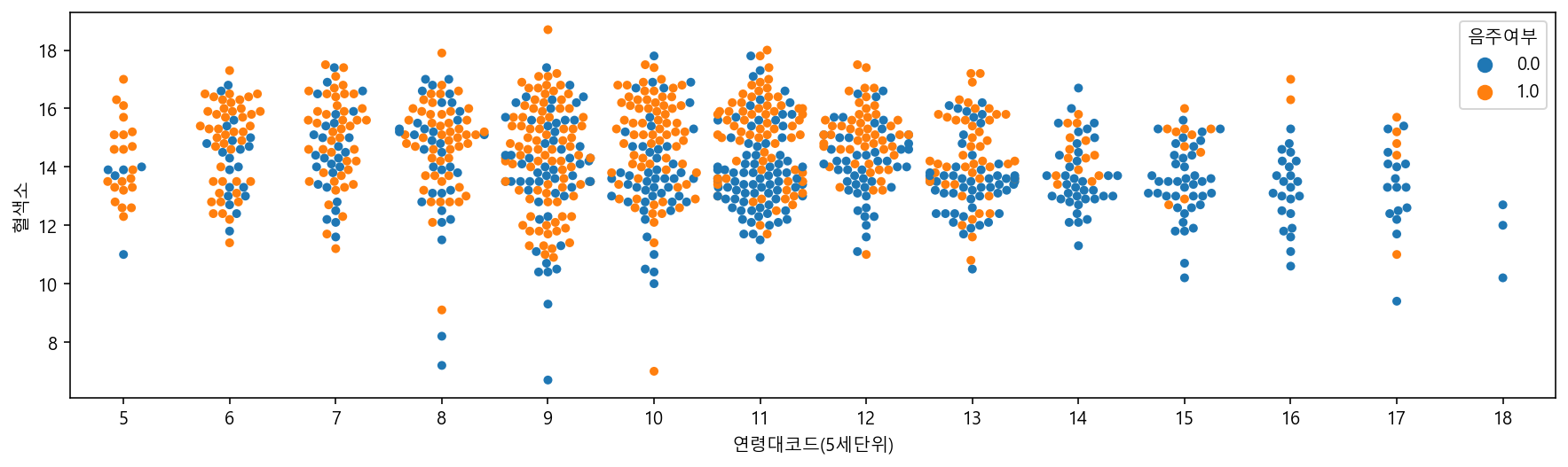
# lmplot 으로 그리기
sns.lmplot(data=df_sample, x="연령대코드(5세단위)", y="혈색소", hue="음주여부")
# 회귀선을 그려서 상관관계를 보여준다.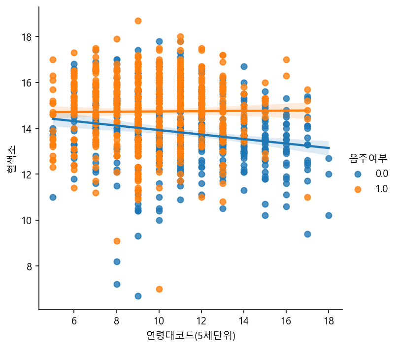
# lmplot 으로 그리기
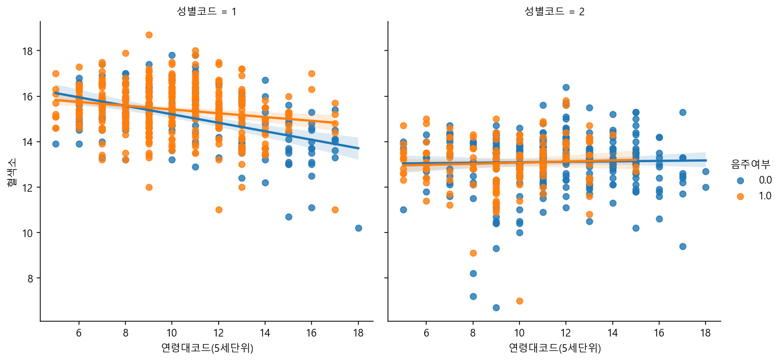
sns.lmplot(data=df_sample, x="연령대코드(5세단위)", y="혈색소", hue="음주여부", col="성별코드")
# 회귀선을 그려서 상관관계를 보여준다.
# col통해서 여러게 나오게 한다.